how to change legend name in excel

Alternatively you can click the Collapse Dialogue icon and select a cell from the spreadsheet. After this click Ok to dismiss the Box.

How To Edit A Legend In Excel Customguide

Spreadsheet 513 views Quickly create dynamic charts 0112 Quickly create dynamic charts.

. Click the chart that displays the legend entries that you want to. Select the cell or range you want to name. You can also click the Add Chart Element button on. Edit legend entries in the Select Data Source dialog box.

Assign the name Legend to the range of legend entries J4J11 in your example and then paste the following code in the sheet module. Imgur link The change will automatically reflect in your chart and the new legend name will appear in the legend on the chart. VbaPrivate Sub ColorsButton_Click Dim c As Range legend As Range f As Variant Set legend RangeLegend For Each c In Selection f ApplicationMatchc. In the dialog set Allow to List.

This box may also be labeled as Name instead of Series Name. After you click OK in the Select Data Source dialog the legend name on the chart will update. The legend name has now been changed to A. Start typing to modify the cell and type in the new desired name for your legend entry.

Create a dropdown list. SpreadsheetGearChartsIChart chart workbookWorksheets Sheet1Shapes Chart 1Chart. By default the Field List pane will be opened when clicking the pivot chart. In the above tool we need to change the legend positioning.

We can select the cell range from A2 to A10 and click the Name Manager in the Formulas tab. How do I change a scope named range. Showing or hiding the gridlines on the Excel chart. In the Edit Series dialog type a new name into the Series name text box and then click OK to dismiss the box.

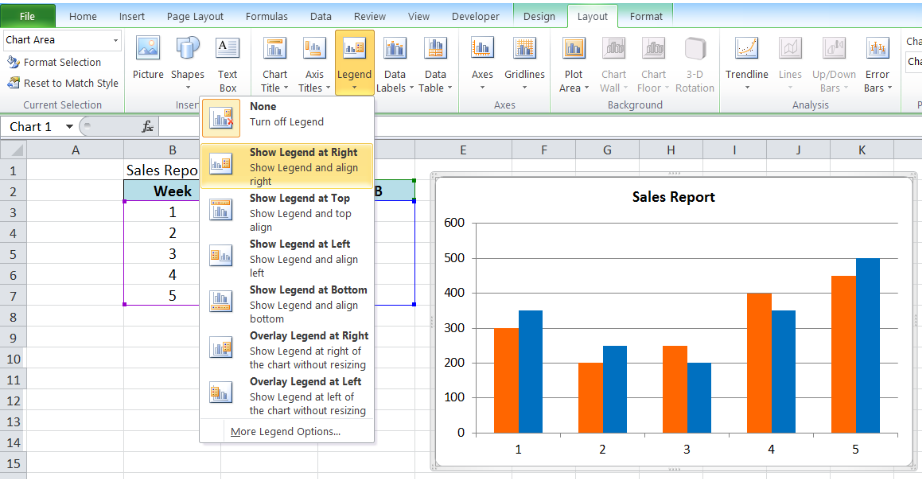
Its shortcut key is CtrlF3In the pop-up dialog box click New enter a custom name select the scope of use and finally click OKIn this way we will give the ce. Click on the drop-down list of Add Chart Element Legends Legend Options. ChartSeriesCollection 0Name My Series Name. Press Enter on your keyboard when youre done modifying the cell.

Select the series Brand A and click Edit This leads to the Edit Series dialog box to pop-up. Select the cells that you want to contain the lists. The new name automatically appears in the legend on the chart. You can then input a custom name for your trendline.

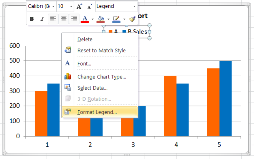
To change the legends formatting you have plenty of different options on the Fill Line and Effects tabs on the Format Legend pane. Type in a new entry name into the Series Name box. SpreadsheetGearIWorkbook workbook SpreadsheetGearFactoryGetWorkbook CChartxlsx. Formatting an Excel Legend.

Delete the current entry Sheet1C2 in series name and enter A into the text box. Click in Source type the text or numbers separated by commas for a comma-delimited list that you. Be careful not to click the word Legend or it will turn it off just hover over it until the list arrow appears. In the Select Data Source dialog box under Legend Entries Series select the data series and click Edit.

Select the Pivot Chart that you want to change its axis and legends and then show Filed List pane with clicking the Filed List button on the Analyze tab. Select the chart Click the Chart Elements button. Select the chart and go to Design. This is found on the left of the dialog.

Double-click the text field delete the current name and enter the name you want to assign to this entry in your charts legend. Click the Options tab. Select a position for the legend. Now pick the legend name that you want to change from the Legend Entries or the series list.

Remove the marker and line from the dummy series so only the title remains. Ad Advertisements L Luke M Dec 15 2008 2 Go to Chart - Add Trendline. Another way to move the legend is to double-click on it in the chart and then choose the desired legend position on the Format Legend pane under Legend Options. After this click on Edit Button and eventually type a name into the series name text box.

By default the legend text is based on the column headings in the data on which. Using SpreadsheetGear for NET you would do it like this. Click on Define Name in Formula tab of the toolbar. In this video I demonstrate how to change the legend text in an Excel chart.

If you are using Excel 2007 2010 positioning of legend will not be available as shown in the above image. Under Design we have the Add Chart Element. Create a dummy data series to add the legend item 3. Open Excels Format Legend pane by right-clicking the legend in a chart and selecting Format Legend Click the windows Fill and Line icon shaped like a paint bucket followed by Fill Click the Color drop-down menu to view a list of colors.

Change legend name Change Series Name in Select Data 1. Right-click anywhere on the chart and click Select Data 2. Delete the tendline legend entry 2. On the worksheet click the cell that contains the name of the data series that appears as an entry in the chart legend.

Changing the legend name with the dialog will not change text in the column that contains your data. Use the Select Data Source feature. Click the Legend button. On the ribbon click DATA Data Validation.

Edit legend entries on the worksheet. How to Make Excel Change Scope of Named Range. Click the Placement tab to change where the. In the Series name box type the name you want to use.

Type the new name and then press ENTER.

How To Change Legend Text In Microsoft Excel Youtube